
The art and science of modeling returns of financial assets is forever unsatisfying because no one model fully captures the true behavior of asset performances. As a result, there comes a point when researchers are forced to pick a poison that appears less wrong than the alternatives. Subjectivity on this front is unavoidable for any number of tasks in portfolio management and design. From simulating to forecasting and beyond, every modeling exercise in finance tends to come down to using a set of approximations that don’t offend our expectations too harshly.
As a simple example, consider the distribution of US equity market returns. Are they normally distributed? The answer depends on the time window. In turn, the implications cast a long shadow on what you can, and can’t, reasonably achieve with modeling.
Consider how one-day returns are distributed via SPDR S&P 500 (SPY), an ETF proxy for the US stock market (based on data for 1993-2022). In the chart below, it’s clear that returns are basically symmetric around 0. SPY’s one-day performances don’t exactly match a theoretically pure random distribution (red line), but they’re close enough so that most of the time, and for most modeling applications, you can assume normality prevails.
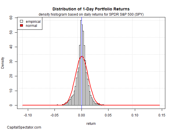
Source: Capitalspectator.com
This assumption has a wide range of implications. For example, if one-day returns closely follow a normal distribution, forecasting one-day returns is futile, at least most of the time. But there’s nothing normal about the one-year return distribution for SPY, as the second chart reminds. The results are positively skewed and there’s a clear incidence of fat tails. The one-year distribution, in short, tells a very different story from one-day returns and so the opportunities for this time window are quite different vs. one-day results.
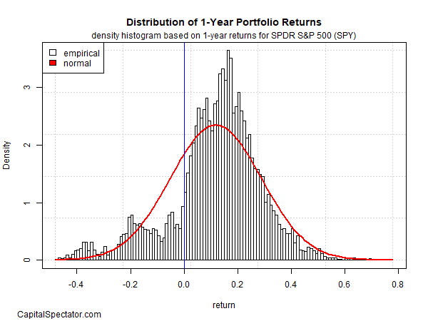
Source: Capitalspectator.com
As one example, the difference implies that one-year returns provide the basis for relatively reliable forecasts. You don’t need a Ph.D. in finance to see that your odds are forecasting success are considerably higher with a one-year time horizon vs. one day. Or perhaps it’s more accurate to say that you’re likely to be less wrong with one-year forecasts vs. one-day estimates.


